Data Insights

Using a dataset obtained through: https://data.world/crowdflower/brands-and-product-emotions, I processed the data obtained from Twitter. Preprocessing the tweets before creating a neural network I was able predict the sentiment using term frequency vectorization.

The dataset is unbalanced.

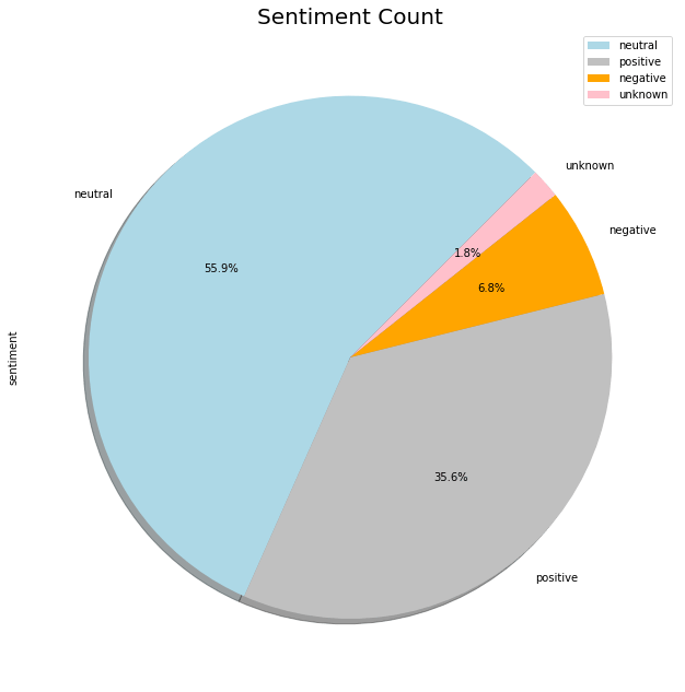
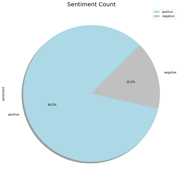
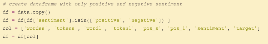
When I opt for binary classification using only positive and negative sentiment categorized tweets, my data looks more like this:

I will consider oversampling the negative data points a little later. First, to clean up the data before I utilize it.

I start by cleaning up the missing data. After cleaning up the NaN/missing data, I had tweets formatted like, well, your typical tweet as seen below.

I also renamed the columns to make my life a little easier.

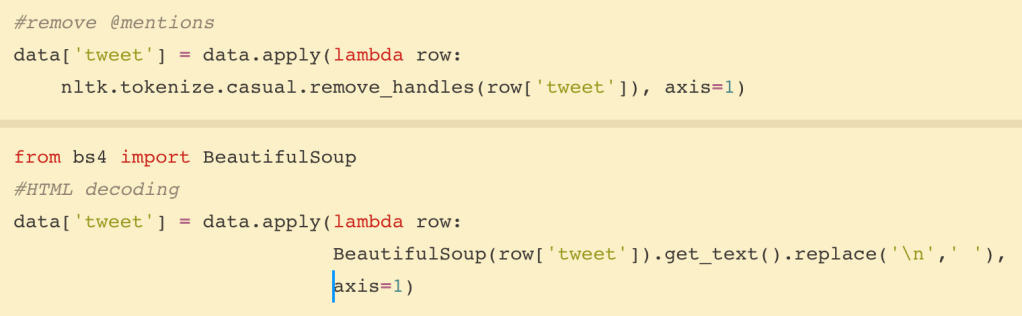
Then, I applied the following functions to my dataset to get rid of the @mentions(Twitter user handles) and to decode the HTML, I used BeautifulSoup.

There were a lot of contractions present in the tweet text, so I used a dictionary to expand them into their compete words, most of which will be removed later through stopword removal. In order to get rid of the hashes preceding the hashtags, websites, auto-populated ‘{link} ‘ text, punctuation, string formatted numbers, possessive apostrophes and extraneous spaces, I applied the following function to return cleaned up text.

Next, I assessed the NLTK stopwords list and decided to add the brand and products to the stopwords and to remove ‘not’ from the list in the case that later, when I apply the n-grams parameter to my process, ‘not’ combined with the surrounding terms could help my network perform better. I also removed ‘sxsw’, and ‘austin’ because the dataset relates to the SXSW event in Austin, Texas. I didn’t want this to affect my assessment of the terms related to sentiment.

I used the NLTK TreebankWordTokenizer and TreebankWordDetokenizer to quickly create columns with tokens as well as an identical column that just contained the terms in a non-tokenized form for later use in Keras, eliminating the need for multiple list comprehension calls in my code. Additionally, after comparing the SnowballStemmer and the WordLemmatizer, I opted to use the lemmatized tokens, as when I applied the Part-Of-Speech tagging, the lemmatized terms allowed for more accurate tagging of verbs.

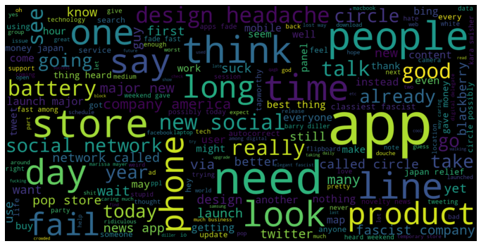
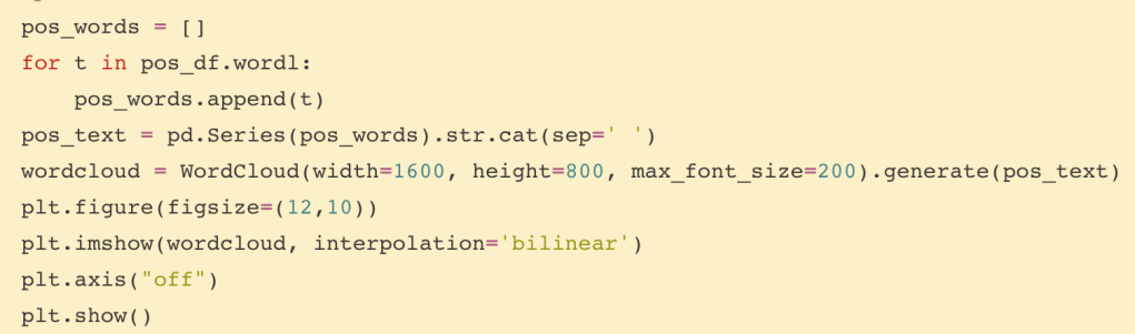
Next, I wanted to get a good visualization on the most common words in both the negative and positive sentiment categories.

I processed my entire dataset, including the neutral and unknown sentiment categorized tweets. Next, I create a new Pandas dataframe that only contains the categories I plan to assess, which is positive and negative sentiment categorized tweets.

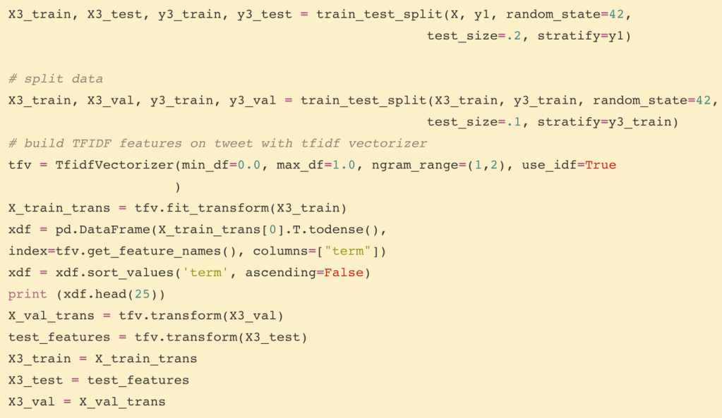
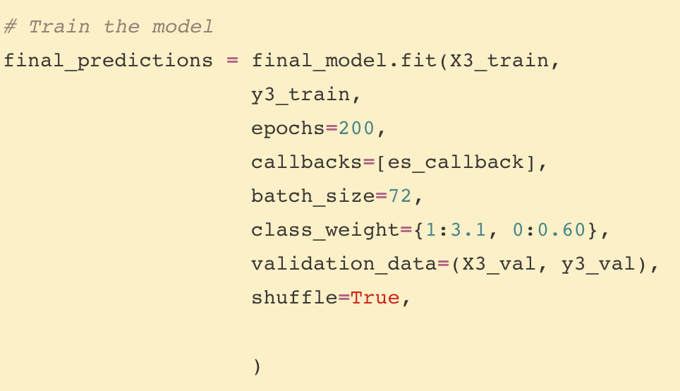
Now, I begin my model process by splitting my data into train, test, and validation sets. Then, I fit the TfidfVectorizer to my training data, and transform all of the data according to the fit to the training data. Then, I get the class weights for the sentiment classes to plug into my compile step.

Now, I compose my model.

I use the class weights when I fit the model to the training data.

My results aren’t bad considering the balance of data, and the overlapping that occurs within the classes.

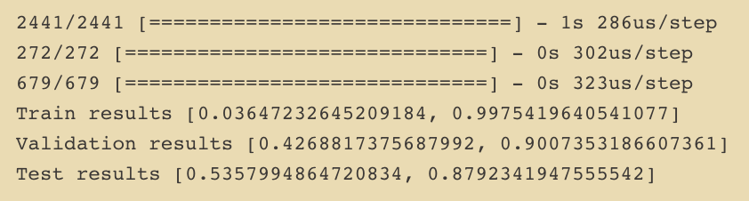
My next step is to obtain more data so that I can assess how the model performs on a larger and more varied dataset. Further assessment to be done on the means and word embeddings as well.

XGBoost has been the leading algorithm for competitions for the past 5 years.

XGBoost is an ensemble of decision trees using a gradient boosting system. The difference between XGBoost and Random Forest lies in the structure of the trees. Fully grown decision trees grow in the random forest based on subsamples of the data, growing and expanding. The larger the tree, the more likely overfitting. Each tree is higly specialized to predict on its subsample. To achieve highest accuracy, the tree continues to split into nodes and leaves as parameters dictate allowing overfitting.

The test set below

Altering these parameters, allowing for shorter trees, distances the potential for overfitting, but at the sake of accuracy. This model below performs at 89% accuracy where as the above model performs at 93%. The change occurs in the parameter ‘max depth’ . This narrows the information that can be processed, therefore limiting the potential for accuracy and also overfitting.

My motivation for the analysis of the King County Housing Dataset is a project for Module 2 of the Flatiron School Data Science program. I was provided a dataset with the below information included.

To start off, I began researching and assessing the dataset. I began by going to the King County, Washington website, https://info.kingcounty.gov/. Here, I found the Residential Glossary of Terms with information regarding the dataset.

Deciding, first, to drop the ‘views’ column, as I do not want my analysis to be tainted by the number of viewings of the properties, as that can be affected by many outside factors, such as realtor’s preferences, buyer curiosity, etc. The number of viewings does not suffice as any sort of accurate predictor or indicator.

Additionally, I reviewed the documentation on ‘grade’. Homes that have grades between 1 and 5 do not meet building code by law. Due to this information, I dropped homes falling below this specification, as I am only including homes that are fit to live in for this assessment. The lower graded homes are more consistent in their value and the higher grades, 11-13 have a wide range of price values but there are fewer occurrences of these grade values occurring overall.

Next, I assessed the ‘condition’ column, and due to the documentation on this description, I dropped any homes rating 1 or 2, only accepting average (needing work, still), and better homes.

I have also opted to drop the “waterfront” information, as there were several NaN values, which could indicate that it is not a waterfront property, but many of the properties already had a “0” for this, as this is already a binary column. To avoid misinterpreting the missing values, as there are 2,376, I simply dropped the column completely.

The “yr_renovated” column also had several missing values, which I interpret as these homes having not been renovated, so I replaced these with “0”. Using this information, I assessed what occurred to my target variable(‘price’) under circumstances where home was renovated vs not renovated. Finding that should the home be renovated, one can price the home over $60,000 higher than those homes of similar grades are priced.

I extracted the year of sale from the ‘date’ column, by converting to DateTime object, then using the year the property was sold and the ‘yr_built’ column, I calculated the age of each property. Then assessed the possible ‘historic’ homes, which, according to the state of Washington, is 50 years old and greater, and retaining the original structure and aesthetics. Since I could not assess the aesthetics, I simply assessed the renovated historic homes vs the non renovated historic homes as far as value. The renovated homes tend to fetch a higher price on a fairly consistent basis.

Next, I began my assessment of the features starting with the bedroom count. There seemed to be some typo errors present, which I corrected, and found that the most common home has 3 bedrooms, followed by 4 bedrooms.

The dataset provided was not in metric values, rather it was in the english system, so I converted all measurements from square feet to square meters.

Deciding to utilize the longitude and latitude information provided, I obtained the latitude and longitude coordinates for the nearest city, Seattle, the used geopy to convert the latitudes and longitudes to a point so that I could calculate the distance from each home listed to the city of Seattle(using kilometers, of course).

I, then assessed the zipcode column and created a graph to visualize the zipcodes and the mean price of homes in each zipcode, before removing the column, along with the ‘lat’ and ‘long’ columns.

Once I finished cleaning up my dataset, removing the english system measurement data, I began my assessment of my target variable, ‘price’.

Due to the fact that the price data is not a normal distribution, I tried a couple different options to scale and normalize the distribution and ended up setting on taking the log of the price values for my assessment.

Some columns that I dropped throughout my assessment include ‘floors’, ‘sqm_lot15’, ‘views’, ‘waterfront’, ‘lat’, ‘long’, ‘date’, ‘yr_renovated’, ‘yr_built’, and ‘zipcode’. Some of these were used to create new data(really, data from a different perspective), some were irrelevant, and others were simply redundant.

Once I completed my data scrubbing and cleaning. I used my variables to get an idea of where I stood on my regression before processing the categorical variables such as bedrooms, bathrooms, condition and grade.

As predicted, there are some issues with some of the data, so I created dummy variables for the categorical data. Rather than keeping all of the quarter and half bathroom values as decimals, I rounded the bathroom values before creating dummy variables(I actually did this both ways and rounding had no negative effect, but allowed me to work with fewer dummy variables). For the dummy variables, I dropped the first variable for each category to ensure I avoided the dummy variable trap.

My continuous data, are as follows: square meters living area(‘sqm_living’), square meters living area of the 15 nearest neighbors(‘sqm_living15’), square meter lot size(‘sqm_lot’), distance to seattle(‘distance_seattle’), and age variables.

Getting closer to where I need to be with this model. I am going to drop the sqm_lot column from my next model. Now I perform stepwise selection based on my p-values to decide what columns to keep.

I then split my data and create a model in scikit learn using the same data.

My model is still overshooting predictions.

To further hone in on the accuracy of the model in the future, I will probably run the square meter data through the StandardScaler() and assess the other continuous data to decide what my best option is for it as well. Additional work as far as Polynomial Regression for the independent variables should also be explored.

For the Mod 1 project, the problem posed is as follows: Your team is charged with doing data analysis and creating a presentation that explores what type of films are currently doing the best at the box office. You must then translate those findings into actionable insights that the CEO can use when deciding what type of films they should be creating.

Using one dataset that was provided, as well as finding a dataset on Kaggle.com, I decided to focus on recent movies, from 2009-2019. Combining these datasets using Pandas, I did profit margin calculations and also created some more palatable number visualizations without scientific notation for the presentation.
As I am analyzing the potential for success, and money is key for most corporations, I focused on domestic gross, because it directly correlates with the international gross, and should be accurate as far as the predictions and assessments made here.

As you can see, the correlation coefficient (using the Pearson method), is 0.94(yes, I am rounding here), which shows a strong relationship. Additionally, you can see that the production budget and domestic gross show a correlation coefficient of 0.73(rounding, again), which shows a moderately strong correlation, so it makes sense that the international gross(also known as worldwide gross here), shows a 0.79 correlation coefficient, which shows an even stronger correlation, which makes sense since the international and domestic grosses show a positive correlation.

After cleaning and combining several datasets, I opted on the two mentioned above, as with their powers combined, I had (or at least thought/hoped I had) everything I needed to complete the analysis that I was aiming for.

Defining success involves monetary earnings. Therefore, I assessed the profit margin, as the production budget for film making has a large range as shown here.

The production budget inevitably affects the gross, as the more spent on a production, the more has to be made at the box office to cover the costs before profits can be earned. The production costs come from the production company starting during pre-production, and if the movie doesn’t do well, but it cost millions of dollars to create, then the production company is at a deficit. But if the movie costs less to make, but is successful at the box office, then the company will be earning revenue much more quickly.

The highest grossing movies in the U.S. do not necessarily make the most profit for a company. As you will see here, action movies tend to earn the highest gross numbers at the box office. The following graphs were created using the top 50 domestically grossing movies from the 2009-2019 dataset. Some of the movies from this subset include the following:

Avatar, Black Panther, Avengers: Infinity War, Jurassic World and Incredibles 2.

These movies make billions and millions at the box office. However, they do not have a high profit margin, due to high production budgets.

I then checked the 50 most profitable movies using the 50 movies with the highest profit margin from the 2009-2019 dataset, and found that the genres that tend to make the most profits for a company are not the same as the highest grossing genres.

Additionally, these movies do not bring in the same amount of revenue as the high grossing movies(by definition, obviously).

The profit margin is high here because of low production costs. Examples of movies included in this subset of data are as follows:

Paranormal Activity, Get Out, The Devil Inside, Paranormal Activity 2, Unfriended, and The War Room

Depending on the way success is determined by a production company, this can dictate the types of movies that should be invested in.

Personally, I am all for more well written low budget horror films. Further assessment is required to get the ins and outs of creating a low budget movie that will sell a lot of tickets. Even more research is required to assess how to create a movie that will not only make profits, but be appealing to audiences.