Recently, I was asked to complete a linear regression task. I was given two .csv files, merged the two files, and cleaned up the data points using pandas. The dataset has the following information:
1) the country
2)the year
3)the dependent variable provided to me is in percent format, representing the percent of total GDP accrued through taxes
4)the independent variable provided is also in percent format, representing the share of population considered ‘urban’
I was asked to do simple linear regression on the two variables, so I attempted to find a direct linear relationship between the unaltered data, and due to the nature of the data, ran into some issues.
Neither of my assigned variables are continuous data, and as I do not have the continuous information such as total GDP, or total population, this information is not enough to find a linear relationship including a constant that makes sense for the almost 5000 data points.
I attempted to groupby the country and scale the data that way, since the percentages are in fact, per country and not percentages of total GDP for the global economy. This did not work either, and my results continued to be poor on the training data. I log transformed the dependent variable, which did not normalize my data, nor did it provide better results, if anything, these were worse.
After getting R-squared results below 0.2 consistently, I decided to add the categorical data, the country value as categorical, dummy encoded data. This gave me an R-squared value over 0.8, showing much better results.
Basically, the linear regression problem in question can not be completed without the total GDP information. Additional data is needed to complete a task such as this, with percentage data as the only variables offered.
Scraping linked in profile and automated personalized connections.
Previously, I posted about using Selenium’s WebDriver to automate the sign in process, scrape user profile headers, job experience, and education history. Once this information has been obtained, it can be used to create a ‘personalized’ message, and Selenium enables you to automate the entire process.
I am beginning this process assuming that the WebDriver instance has been created, as ‘driver’, in this case, and the sign in process has been completed using Selenium, and if you need a refresher, check out ‘Web Scraping #1’, and earlier blog that details this process.
Once you’ve logged in, just point the driver toward the linkedin profile url.
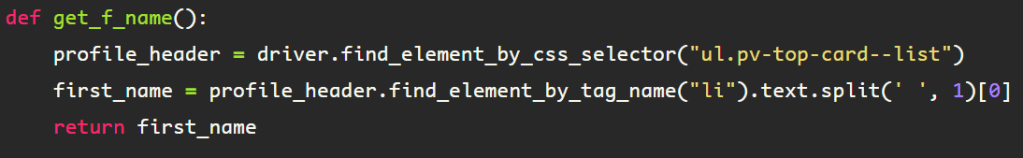
The following function is used to get the first name from the profile, and is built using the foundation of the ‘get_name()’ function from the ‘Web Scraping #2’ blog. First, the element containing the user’s name from the profile header, under the </ul> tag, class name ‘pv-top-card–list’, then from there, find the </li> elements, note the singularity of the find_element call, as this is all that is necessary to extract the first name, which is all I am using for compiling the ‘personalized’ message.
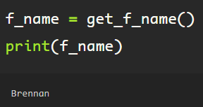
Run the function, assigning the returned value (first_name) to the variable ‘f_name’. Here, to validate that the function works correctly, I printed the ‘f_name’ value.
For this particular connection, I am using the ‘get_education’ function from ‘Web Scraping #4’, in which I went through the process of extracting data scraped from a user profile, including the experience and education section. This is to show how the information extracted can be used in the ‘Connect’ automation.
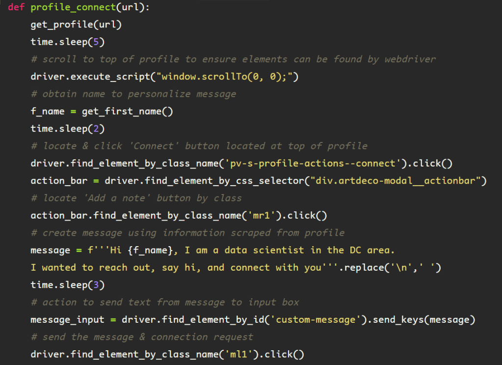
Next, I am going to direct the driver to scroll to the top of the webpage with the following line of code. I am doing this to ensure that the element is available to the Selenium WebDriver due to the dynamic nature of LinkedIn’s webpage build.
Contained within the profile cover, there lies a banner with basic information on the left side of the screen. On the right, are buttons with which the web driver can interact with Selenium’s ActionChains simulating a mouse click with ‘click()’.
First, the ‘Connect’ button is located by directing the driver to the class element belonging to the button seen on the screen, followed by the click() function, this emulates a mouse click on the button.
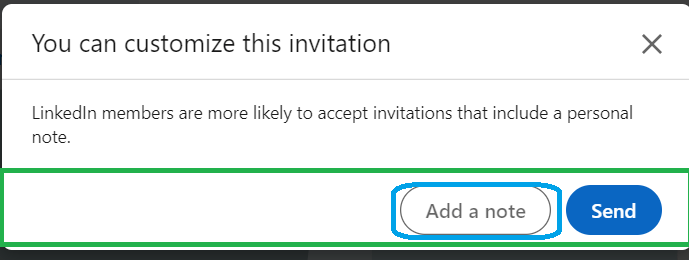
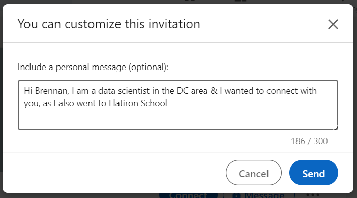
The next window appears after the click, and the goal is to click() on the ‘Add a note’ button, circled in blue in the image below.
To successfully locate the button, first, point the driver to the element tag</button> including the attribute ‘aria-label’, and click() it, which will prompt a new window with a text input field for a customized invitation.
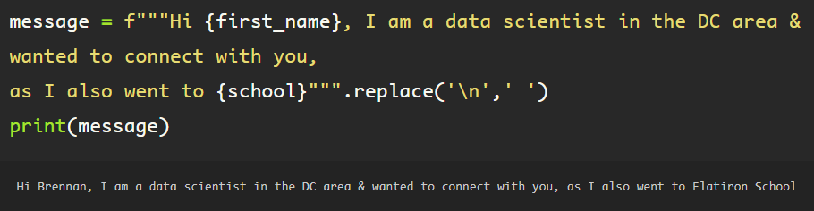
Using basic python string formatting, create the message to be sent with the invitation.
This message is formatted and assigned to the variable ‘message’ and ready to be sent to the customized invitation input.
Locate the ‘Send’ button and click it to simulate the mouse click.
The message has been sent, and the window closes leaving the driver on the standard profile page.
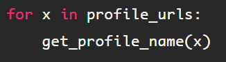
This process can be encapsulated into a function, making it easier to use when iterating through a list of urls. Changing the method used to locate the ‘Add a note’ button, instead, finding the container containing the element, then locating the element by class name, rather than through the attribute used before. This is due to timeout and element not found errors that occur when the previous elements are utilized in a loop.
Continuing the long road that is scraping LinkedIn profiles with Selenium
LinkedIn contains a wealth of information for a large community of working (or looking for work) professionals. Up until this point, I have gone through the process of automating the sign in process, scraping search results, and the basic process that starts off the profile scraping task, getting the name of the person who’s profile is being scraped. Now, I will go in depth, scraping contact information, job experience, as well as education experience. This are all details that could prove useful when one wants to connect with individuals from a specific company, in a specific role, or with fellow alumni.
Since the log in process is automated, I am simply going to use that to sign in, which I went through in the first blog of this series, but here is a visual recap, in which the WebDriver instance is created as ‘driver’, the log in process is defined as ‘sign_in’, requiring email and password inputs as strings.
This walk through is going to be on an individual URL(provided as a string), but this can be used to loop through multiple URLs to scrape multiple profiles.
LinkedIn, as well as a plethora of other websites utilize AJAX programming, also known as “Asynchronous JavaScript and XML. This is a method of dynamic programming that creates a smooth user experience for the normal user, but proves to be a huge pain for web scraping. The elements load dynamically as the user manually scrolls the elements into view. So, if the information is in the middle of the page, there may be errors preventing the ability of Selenium to extract the data. For example, when directing the WebDriver instance to the experience section of the profile, because I simply loaded the profile, which only shows the top of the page, before scrolling down, only that CSS information is available to my driver.
Theoretically, this should work, however, I get the following error.
Fret not! There is a solution to this problem. First, I am going to locate an element located higher up the tree. I am selecting the following element, labeled ‘background’, as it is a larger component, that encompasses the elements that I wish to obtain. Then, I scroll this into view using a JavaScript command.
Now, I am able to get my ‘experience’ section. I will later be able to use the ‘background’ element to find the ‘education’ section, so it’s a two birds, one stone situation.
Moving onto job history, which I obtain by finding the elements, note the plurality, that are under the a-tag shown in the coding block below. Next, I define ‘details’ as the first element in the list of elements, which is each job block under the ‘Experience’ section on the profile.
If I want to get the information for the second job, I would simply alter details=history[0] to details=history[1], but I am just using the first job for this example.
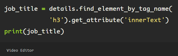
Now that the first element in the list has been assigned to the variable ‘details’, I can get the job title, company name, and any information that exists within this job block. Using the ‘get_attribute’ method, I am simply grabbing the ‘innerText’ to get the user’s job title.
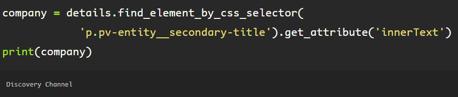
A similar format is used to obtain the company name for this job.
Then, to get the dates, again, finding the correlating attribute to the css selector referenced, which provides extraneous text that I do not need.
This is something that Python allows me to remedy easily, by splitting the list on the second white-space separator, which occurs after ‘Dates Employed’. Then I specify that I only wish to use the string in the last position of the list, of which there are two elements. Now, I am able to get the date range for this job.
A similar format is used to get the education information from a profile. Using the ‘background’ object defined earlier, simply locate the education section, using the WebDriver, pointing it to the element on the page.
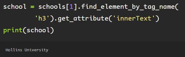
The ‘schools’ object is a list which is iterable, just as the job ‘history’ object from the experience section earlier. Following a similar flow, simply extract the ‘innerText’ attribute from the ‘h3’ tag, which provides the text from the first h3 tag, from the first element in the list (schools[0]), note the singularity the ‘find_element_by_tag_name’, otherwise, if element is plural (elements), a list would be returned, if there are multiple ‘h3’ tags inside of the first school object, which I do not want in this case. You can see here, the output is a string, and the name of the first college in the education section.
If I wanted to get the second college from the schools object, I’d just change up the number representing the element in the list ‘schools’.
In addition to getting the experience and education for a person, I’d like to obtain the email from the contact info section on the profile. Since this is located in the header just under the photo, first I need to scroll to the top, because, remember, LinkedIn uses AJAX.
Now, from the top of the page, under the profile photo and header info, there is a blue hyperlink that says ‘Contact info’. Pointing the driver toward the a-tag element using the ‘data-control-name’ attribute contained inside the tag, Selenium makes it easy to just click this, which prompts a pop up window with the person’s contact info, including the profile which I am looking at as well as the email for the person, should it be provided.
Using the WebDriver, I find the element holding the email, extracting the ‘innerText’ attribute’s information, I am able to get the email in string format.
Now, I can put each into a function of their own, using the try/except blocks that make Python so brilliant in cases like this, because not all people include all of the information in their profile, which would cause an error, halting my code. In my ‘except’ clause, if the element is not found, rather than an error, now, it simply returns ‘nan’, so when I run the code on multiple profiles at once, without getting hung up on an error.
Scraping individual Linkedin profiles for information.
Previously, I went through the process of automating your Linkedin login, and scraping potential connections after automating the search from the homepage post sign in.
I will start by creating the Selenium WebDriver instance, calling it ‘driver’.
Then I will log into my linked in account using the process detailed in the first blog on web scraping Linkedin.
Next, I will assign the url of a profile, as a string, as variable ‘profile’, followed by the line telling the WebDriver to ‘get’ the url.
Once the profile page loads, you can see the person’s first and last name below the photo in the profile header. I am going to grab the name of the person to ensure everything matches up should I decide to process in batches later.
Upon inspecting the HTML for the element containing the name, headline, location and connections information, you see it can be found here:
To convey this to the WebDriver, I create an instance called ‘profile_head’, finding it using the css selector using the ‘ul’ tag and the class ‘pv-top-card–list’.
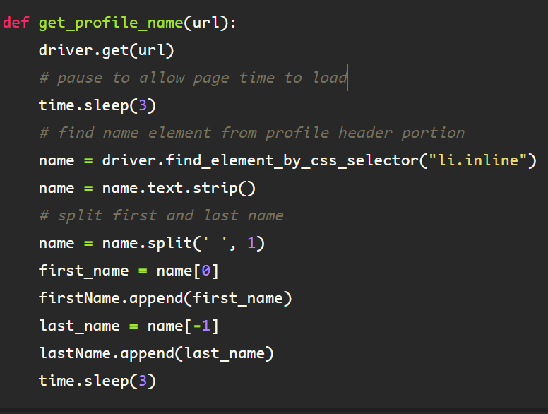
Then to get the name from the element, I simply find the first element under the above tag using the list tag ‘li’, class name, ‘inline’, as the first occurrence contains the innerText attribute containing the name string. I assign the variable ‘name’ to this.
From here, I got the text from the element, and split the string on the remaining center whitespace, which separates the first name from the last name in a list, from which I extract the variables ‘first_name’ and ‘last-name’.
This process can be combined as a function, then you can iterate through a list of Linkedin profile urls, which can be extracted by following the process outlined in my previous blog, Web Scraping #2.
Using Selenium for web scraping jobs, connections, etc.
Back in Web Scraping #1, I walked through how to automate the login process for LinkedIn. So, now that we are logged in, the fun begins with Selenium. I am going to walk through searching LinkedIn and scraping the search results page.
This process picks up immediately after you have logged into LinkedIn. If you would rather just login manually ::scoff:: then you can simply create the WebDriver instance, then copy the URL from your browser and paste the URL, don’t forget the ‘string’ notation, so that Selenium can take control of your browser.
You’ll have an instance of the Chrome browser open on your computer, which is indicated by this at the top of your browser:
You should see this search bar at the top of your screen in your browser, which should be controlled by Selenium now.
To understand how the HTML and CSS are functioning on the page, enter CTL/SHIFT/i, or since I know the element I am looking for, I simply right click with my cursor on the search box.
Click “Inspect”. The blue highlighted html text refers to the search bar typehead, which is what we are going to tell our Selenium WebDriver, or ‘driver’, which does not need to be updated if you followed the login process in Web Scraping #1.
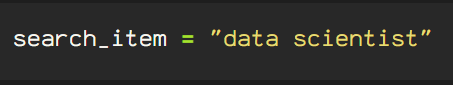
Let’s just go ahead and declare a variable for the term for which we are searching.
Next, we will direct the driver to the search bar. Here, I found the element using the id. Then after locating the element which accepts the text input for the search, using the input tag and class name from the HTML on the page, I then add the Action Chains function ‘.click()’.
So, in the first line of code, I am activating my cursor in the search bar, then, I am simply sending the ‘search_item’ variable, which is the string above containing my search term. This ‘send_keys()’ function enters the keys for my search term. Below, is the result of the code up until this point, which you can see in your automated browser window.
Next, we run this line of code, which sends the ‘RETURN’ or ‘ENTER’ key after the search term has been typed out.
Once this code runs, the browser opens the webpage containing the results for your search. This should have sections such as “Jobs”, “People”, and “Posts”. First, you can define whether you are searching for jobs, people, or posts as the ‘target’ variable. Next, I assign the variable ‘button’ to the element’s link text, which is visible in the banner, but can be verified in the HTML.
target = ‘people’
The second line of code, I use a JavaScript command, because the Action Chains and Python commands prove tricky with buttons or clickable areas that prompt new url windows to open. Now, I am going to extract the information for only the first item returned in the search container for now, but this will all be automated later.
In the first line of code in the next block, I find the first element by specifying ‘find_element’, rather than ‘find_elements’, so, only the first instance of the CSS selector is selected in the class ‘entity-result__title’, which is referring to the box that contains the name of the person on the profile. Both items I need are located here, for now.
In the second line, I basically piggy-back off of the first line, so now, the WebDriver is only retrieving information from the first search result, due to specifying ‘result’, where previously ‘driver’ was the instance. Additionally, I split the string, so a list is returned for the result, including the person’s name field as text[0], and as text[1] contains the string “View (name)’s Profile”. These are located within the HTML/CSS for the ‘result’ element, under the attribute “innerText”. This is verified with a simple ‘print’ statement. For the person’s linked in profile url, the attribute which contains this is the pathName attribute, again verified by a ‘print’ statement.
The primary and secondary subtitles tend to be populated by the company where the person works and their geographical location, which I located using the ‘css_selector’ correlating which each. For the primary and secondary details, aka ‘deets’, I am no longer using the ‘result’ element from earlier, due to the fact that it is just the ‘title’ line of the individual search result and it’s corresponding </a> tag.
Here is the output for the above code. This is exactly what I am looking for. Next, I will create a function and incorporate pagination in my automation so that I can get hundreds of results, add them to a Pandas DataFrame, so that I can assess the data, and then filter and decide which profiles I want to fully scrape and connect with in the next installment of “Web Scraping”
For a quick extensive search, a loop can be implemented.
Web scraping is a great way of obtaining data, but with all of the data available, doing it efficiently is another story. I am starting my web scraping journey by using LinkedIn’s search function to find connections, as I am a relatively new professional in the field of data science, and with 7.8 billion people on the planet, “who” you know can be almost as important as “what” you know, and deciding what data to extract beforehand will save me a lot of self loathing down the road. This is the first in a web scraping series that can get anyone started with web scraping and automation in data collection.
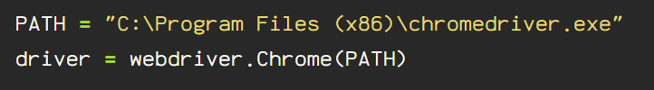
To get started with Selenium, first we have to get a driver, to interact with the webpage, or ‘to drive’, essentially. I used Chrome, and the correlating driver is found here: https://chromedriver.chromium.org/. There are separate drivers for Firefox, Explorer, Safari, and a handful of others, just check the Selenium WebDriver Documentation for more info. Once this is downloaded, just unzip the download, and place the chromedriver.exe file where you’d like it to live, assuming that you’ve already installed Selenium using pip, import the following basics to begin with:
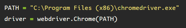
Next, define the path to the driver.exe file and define your driver, be sure your browser and driver executables match or you’re done before you get started.
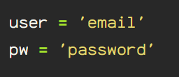
Now that you’ve got everything set up, we begin actually working with Selenium. First, create & store variables containing the user’s email as a string datatype. Do the same with your password.
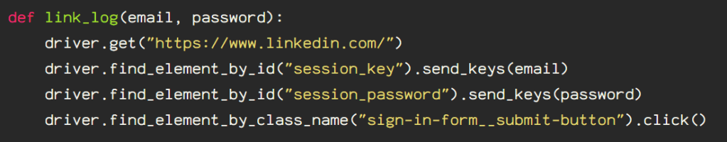
The first line in the next part, which is actually used to log in and enter the password provided. The driver ‘gets’ the site. Next, the driver locates the id called “session_key”, the ‘.send_keys’ command is pushing the email string in the email input box to log in. The ‘session_password’ id input variable is the password assigned variable. Finally, the ‘sign in form’ button, which is div class ‘sign-in-form__submit-button’, which has the ‘click()’ action performed on it, simulating a mouse click.
Once this is run, you will have a Chrome window open with your linked in account logged in and ready to go.
There are various ways to display data, but there are a few things to consider before creating a graph to convey to that data to someone else.
Whether it is numerical or categorical, a means to convey the composition of your data is a common necessity.
An initial basic composition assessment is a good place to start with any dataset. Identify the target variable. Composition implies that the samples are from a set or group, with characteristics that differentiate each individual from the larger group, or divide them into subsets through the attribute(target variable) in question.
For instance, say I am assessing the sentiment of a set of tweets. All of the samples are in the larger group, tweets, however, there are negative and positive sentiments associated with each sample, to be used for a classification task. One way to visualize the data is a pie chart, which is effective in this case due to the large difference between the count of negative versus positive sentiment. This shows that the dataset is severely unbalanced, which will require consideration when creating a classification model for this dataset. Pie charts should always add up to one hundred percent.
Side note: When presenting information, always add a title to your graph, even if no one else will see it except for you, even if it’s a super basic title describing the contents of the visualization.
Another way to visualize the composition of data is a stacked column chart. In this chart, you can visualize subsets within subsets, as the y-axis is used to separate the group into 4 individuals. Each individual has read books, nonfiction and fiction, which are shown as percentages on the x-axis. This graph can get confusing for the viewer, due to the orientation of the numeric data axis. For instance, Amilie, roughly 25% of the books she read are nonfiction. The viewer must then subtract that to get the fiction data. It is, however, an impactful visualization for simple comparison purposes.
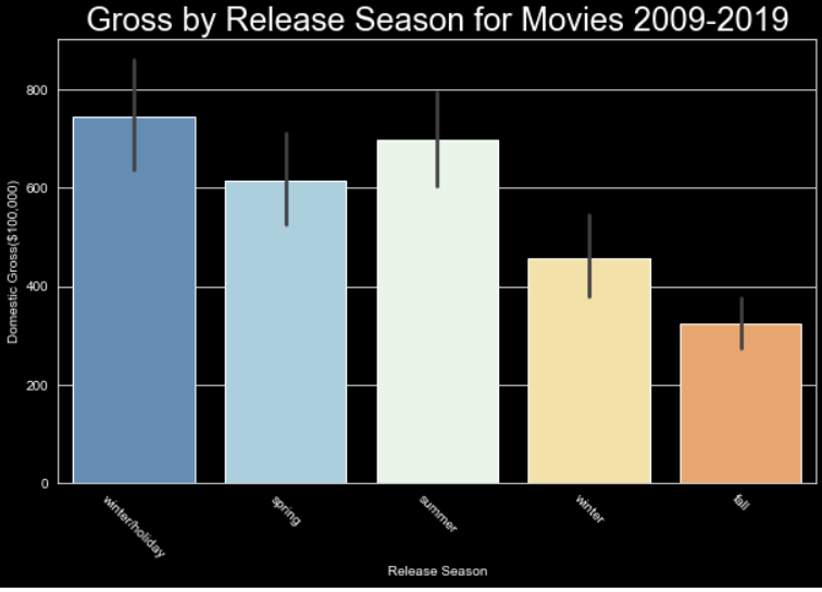
A bar chart can be used to visualize values for categorical variables. The outliers and different quartile ranges can be added as visual options using Seaborn or Plotly, providing an extra layer of information.
Say we want to see the way data changes over time, or to compare two variables within the dataset, one being a continuous variable, we can use a line graph. Line graphs can be used to show change over time, visualize outliers, and compare relationships. Here is an example of relaying information with a line graph. The x-axis shows the age of homes, this is the continuous aspect of the data. The dark blue line is the mean price in the tens of thousands of dollars for homes of the age indicated on the x-axis. The light blue shows the variance within the homes of the age indicated. Line graphs are great for visualizing trends and chart continuous data over time.
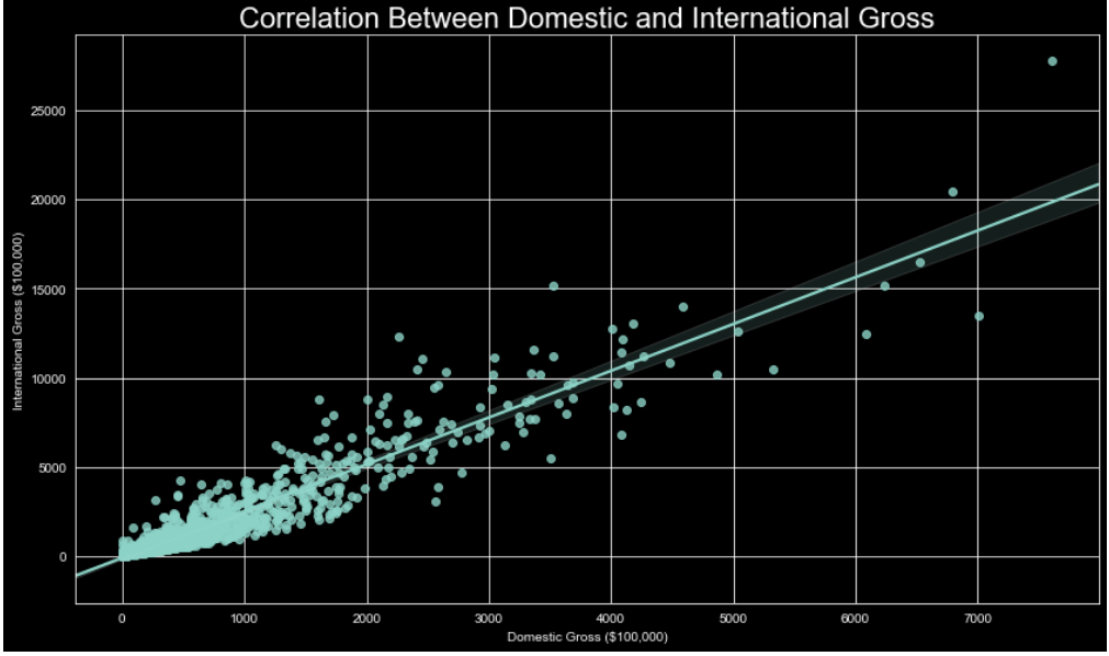
A scatter plot is used to visualize trends as well. Rather than a single line, representing the mean, each data point is placed representing the values of the two variables on the x and y axis for said data point. This is a helpful way to visualize outliers and compare feature correlation.
These are just a few of the most commonly used methods to visualize data using graphs. There are 3 dimensional axis options, flow charts, boxplots, waterfalls, and more, but to truly understand the relationships between variables, these graphs are sufficient for the task, and more robust options are available within these as well.
Eighty to ninety percent of a data science project involves processing the data, this has to happen before any model is fit. Data comes in a variety of disarray, different file formats, empty values, even no formatting. Once you sift through the data, organize it, standardize it, and really start to visualize the data, feature selection can begin.
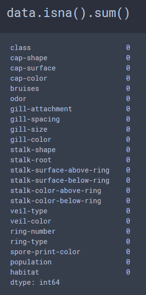
I am going to use the Mushroom Classification Dataset, which provides 8,124 samples, with 23 features for each sample. Unusually, there are no missing values for any of the features for any of the samples in this dataset and the dataset was very balanced, which I rarely encounter.
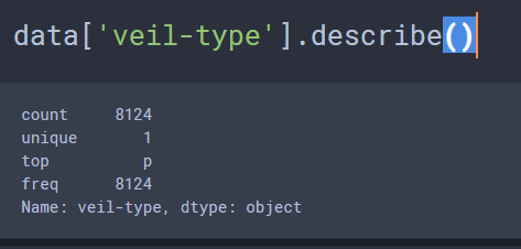
There are a variety of attributes being assessed for the binary classification task of whether a mushroom is poisonous or edible based on these 23 physical characteristics. Actually, lets make that 22 right off the bat, due to the fact that there are two possible values for the ‘veil-type’ attribute, partial=p & universal=u, however there is only 1 unique value for this column, so this column can be eliminated off the bat, due to the fact that 100% of the samples present in this data display the ‘partial’ veil-type attribute.
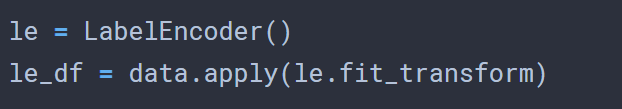
That was the easy part. I decided to try VERY basic feature selection based on the variance and also for correlation, to compare the features selected using each method. Now, since the data is categorical by nature, calculating the variance involves first label encoding the data.
With a quick check on the variance for each column, simply within the column, I chose the 5 columns with the highest variability.
When checking the correlation coefficients for each column based on the feature and the target, the following columns returned the highest correlation coefficients.
When I noticed that ‘bruises’ was present in the second set of features, I had some questions, due to the fact that I am not an expert in mycelium, fungus or mushrooms, whatsoever. I found out that the presence of bruises isn’t what is critical in identification, but the color which the mushroom bruises. The dataset only provides the following regarding bruises: bruises=t, no=f, so it’s simply the presence, not the color. For now, I will leave this alone, however, I will be researching this further.
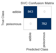
I ran GridSearchCV with a 5-fold StratifiedKFold() for cross validation for both sets of features.
The following are the results for the dataset with feature selection performed using correlation coefficients.
best parameters are: RandomForestClassifier(max_depth=8, n_jobs=-1)
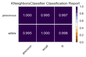
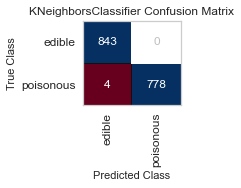
best parameters are: KNeighborsClassifier(algorithm='ball_tree', weights='distance')
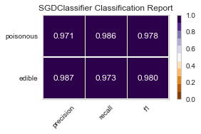
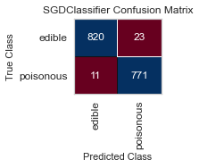
best parameters are: SGDClassifier()
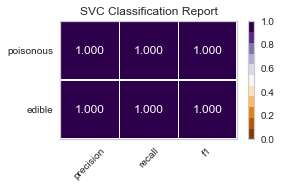
best parameters are: SVC(C=1, degree=1)
Now these are the GridSearchCV results, with the same cross-validation on the variance selected features.
best parameters are: RandomForestClassifier(max_depth=8, n_jobs=-1)
best parameters are: KNeighborsClassifier(algorithm='ball_tree', weights='distance')
best parameters are: SGDClassifier()
best parameters are: SVC(C=1, degree=1)
For both sets of feature selected datasets, I keep running into Type II, False Negative errors, which in this case are detrimental to the person eating the poisonous mushroom, thinking it to be edible. I will be further honing my feature selection, and doing more research to conclude the set of features that minimizes the Type II error for this classification task.
When I ran the same GridSearchCV on my label encoded data, my results for RandomForestClassifier() were far better, as no one was ill advised to eat a poisonous mushroom using all of the features(minus the veil-type feature I removed early on). Perhaps I need to reassess the limit of 5 features to classify the mushrooms edibility, and expand to 6 or 7, as that could be the one missing element.
best parameters are: RandomForestClassifier(max_depth=8, n_jobs=-1)
best parameters are: KNeighborsClassifier(algorithm='ball_tree', weights='distance')
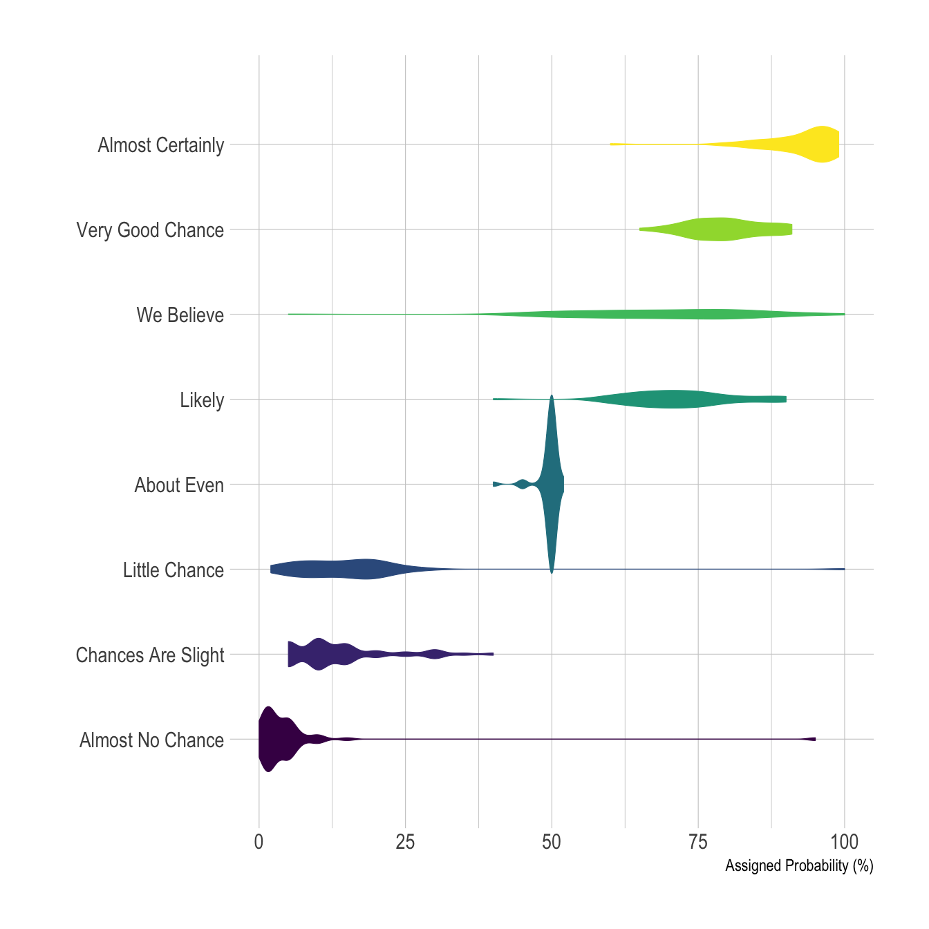
The violin plot is, in my opinion, very underrated. Everyone knows the box plot ( or the box and whisker plot), but the violin plot can do everything a box plot can do, with more style. It’s a great way to visualize density representation, the wider parts of the violin body show a higher density. The outliers are visible from the elongated portions from the top to bottom(depending on the plot, sometimes it’s side to side, see, versatile!). You can even represent your data with a boxplot within your violin plot.
Using the ‘point’ or ‘stick’ parameter, view individual data points. Saturate the color to give a color representation of the density. There isn’t much this plotting system can’t convey. It makes sense at first glance too, so it’s hard to refute the clarity with with the violin plot is capable of conveying information.
Using the ‘hue’ parameter, visualize two variable’s density side by side. Add the quartiles and convey more information in less space.
Orientation is not an issue for, it provides more creative license in conveying information. The heavier distributions are seen as the tall violins, and the wide spread distribution with its outliers, evident as it spreads across the graph’s X axis. The violin plot provides the creator the versatility to condense a variety of information in an artistic way that even the most dense of us can understand.
So, next time you’re creating a presentation, or just trying to visualize data for yourself, don’t lose hope. The violin plot can show you the way.
Audio analysis in machine learning can be done using complete audio timelines or extracting information from certain features. Depending on the end goal, there are a multitude of methods one can use to analyze audio.
Common applications for machine learning in audio classification include speech recognition, music tagging, and fingerprinting. My capstone project was done on audio classification, and I chose to classify bird species based on their calls and songs. I obtained the data from https://www.kaggle.com/c/birdsong-recognition.
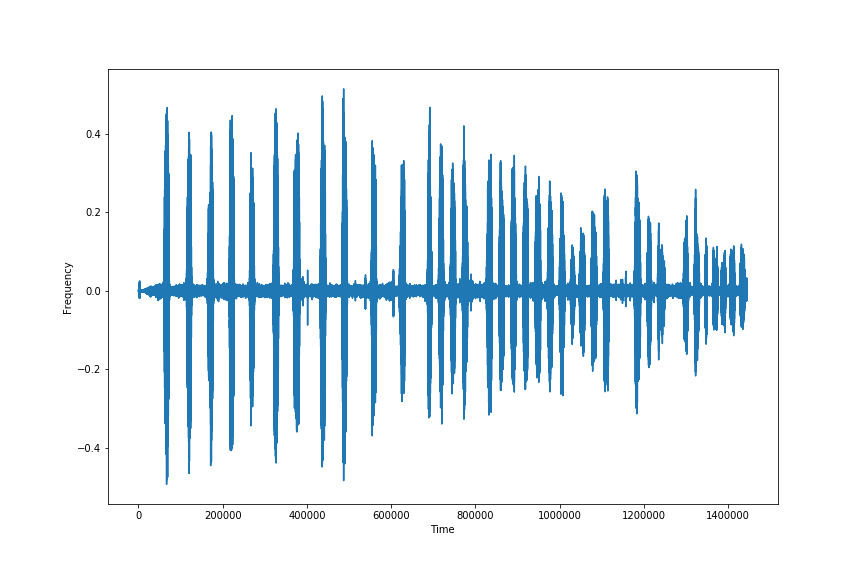
The audio was in mp3 format, and there aren’t a lot of libraries for audio analysis, and Librosa, being one of the most common, requires wav formatted audio files. I started by using the Pydub and Soundfile libraries to convert the mp3 files to wav formatted files. Next, I sliced the files using pydub’s split_on_silence feature. Rather than removing the actual silence, I increased the threshold so as to remove the excess background noise, as there is not only ambient/environmental sound present, but there are squirrels, other birds, and a variety of extra ambient noise present in the audio tracks. I chose the split on silence module because I wanted to actually split the audio track rather than re-leveling the audio, which would change the pitch and quality of the audio files. Below is an example of the information obtained through the wav analysis, which essentially shows the power at certain points and around the 0.0 mark across the center, is the ambient and background noise present throughout the clip.
The above image is the melspectogram extracted from the same audio file. Setting the lifter to 2.0, so as to focus on the power of the audio file, you can see the light pink color that reflects the call of this bird.
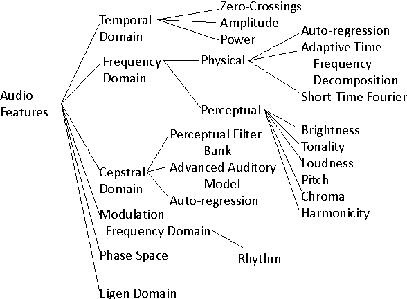
Deciding what features to work with was one of the many hurdles I encountered. There is so much information in sound, from pitch, to frequency, to power. All of these have to be extracted with consideration to the extraneous sound present on a track when it is obtained in certain environments. This was consistently the case for the dataset I worked with for this project.
Since audio is actually linear, I initially intended on sticking with the wav and chromagram information, but upon doing some research, I found that the melspectogram represents audio as human’s perceive it on the log scale. I extracted a variety of information through statistical analysis to utilize in my neural network. I worked with the onset envelope, to get an idea of the power behind the bird call for each file. I assessed the spectral deviation, which involves taking the standard deviation from the chromagram information extracted for each frame of audio. I assessed the mean mel cepstral coefficients from the audio tracks as well. These assist in provided key information on the mel scale through coefficients obtained in a frame by frame analysis.
There is a plethora of audio features that could be used to identify sounds and frequencies.