Image Restoration & Enhancement with Python using OpenCV & Numpy


Machine learning and AI have come a long way with regards to processing images. From visualization, pattern recognition, image restoration, graphics sharpening and search retrieval, it’s become a part of every day life for most primates with a smart phone. For those who directly implement the machine learning tasks, the process involves a much deeper dive.
Starting with image acquisition, followed by enhancement and/or restoration, then morphological processing. These are all done in the preprocessing stages, before feeding the model, customizing these processes for the image data being used can be useful to enable a much faster ML model, since images contain such large amounts of data. It’s not unlike the typical data science process of scrubbing and wrangling the data, getting rid of unnecessary information that will skew or slow down the final model.
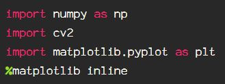
Let’s get started. First, as usual, import the libraries:
Let’s start by analyzing the image using a histogram to get an idea of the pixel layout using the OpenCV built-in histogram function, cv2.calcHist(). Documentation for this can be found here.
Start by importing the image in grayscale, this reduces the channels as we are just looking at the intensity levels of each pixel, and the saturation of color, or lack thereof. This is how we are able to visualize the contrast of the image numerically. Image contrast is defined as the difference in brightness, and the spread of this information is known as the dynamic range.
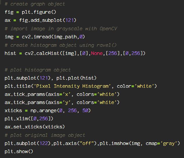
The resulting histogram shows the dispersion of pixel brightness, from black to white and the shades of gray in between.
0 == black, and 255 == white

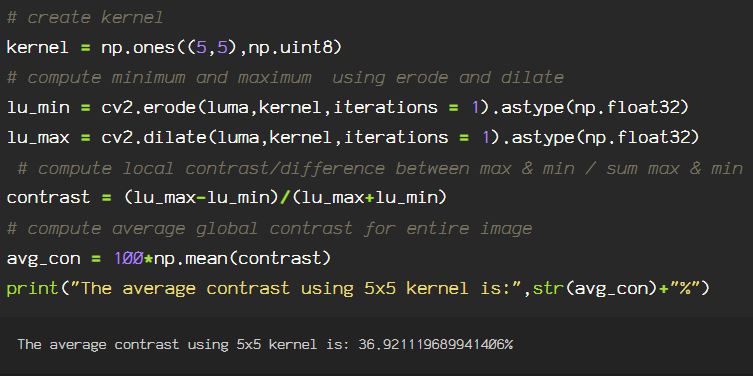
Using OpenCV morphological transformation functions, cv2.dilate() & cv2.erode(). The dilate function provides the growth(aka dilation) of pixel information providing the maximum. The erode function, in contrast to dilate, computes the local minimum. These processes are convolution based, therefore a kernel is created and used to scan the image through the lens of said kernel.
The center of the kernel is the anchor point, moving the kernel across the image gradually, calculating the maximum(for dilate), or the minimum(for erode), and updating the anchor point information accordingly, resulting in the gradual dilation/erosion minimum/maximum.
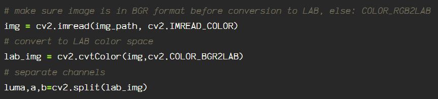
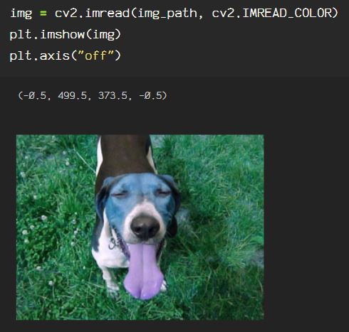
To calculate the average contrast using this method, the image is read into the BGR color space. Next, using cv2.cvtColor(), convert from BGR to the LAB color space, and separating the channels, enables the relevant contrast information to be easily accessible. Remember, the L channel in the LAB color space contains the brightness information for the entire image.
Creating a 5×5 kernel, which is just what I chose, you can chose any size kernel, but know that the larger the kernel, the more information is added to the convolution process.
Some images are just too dark, other times, they’re blown out with light, either way, detail gets lost, and those details are often the most important part of an image in machine learning processes.
There are options for enhancing these images, so you get back as much detail as possible.
One option for adjusting the brightness of an image, either adding or removing shadows, affecting the contrast and lines, is Gamma Correction.

Gamma correction is used to adjust the intensity of each image pixel using a non linear operation resulting in a change to the intensity through relative proportions between the input and output pixel through a power law relationship. This affects an attribute called luminance. This is the human perception of ‘brightness’. Gamma correction on pixels is processing the image pixels by adjusting physical brightness linearly pixel by pixel.
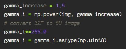
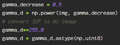
So when gamma correcting, each pixel value (non-negative, between 0-1) is raised to the power of gamma, where if gamma < 1, the perceived brightness of the image is increased, and if gamma > 1, the perceived brightness decreases, but this is due to the saturation decrease, removing shadows when gamma is < 1, just as the intensity of the pixel saturation appears darker when the gamma is increased.
To do this in OpenCV start with cv2.imread() and Numpy(np), converting the pixel information to floats and dividing by 255. Why 255? Because there are 256 color values for each channel (red, green, and blue), since 0 is included, it’s 255 to encompass all 256 values for 8-bit image, the bit depth at which OpenCV reads the image using cv2.imread. Doing this gives us values between 0, 1, so that upon application of the gamma value, this does not impact the numbers so severely, which would blow out or totally darken the image, throwing it out of the color spectrum beyond the black:0 and the white:1. The gamma can be increased, providing more intense colors, or decreased, which brightens the image, removing shadows.


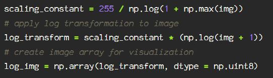
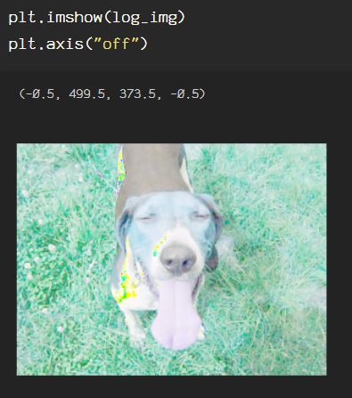
Another transformation, similar to the power law transformation used in Gamma correction, in the log power transformation. Rather than being a linear process, the logarithm of each pixel is used to transform that pixel, instead of each pixel being transformed by the same exponent, the extra step of calculating the scaling constant gives different results from the Gamma correction.
For the log power transformation, I will not convert the data points to floats, rather keeping them as integers ranging from [0,256]. I will just import the image using the standard OpenCV BGR color space.
To apply a log transformation, creating the scaling constant by dividing 255. For the last step, using Numpy, convert the log power transformed data points to an array of 8-bit/unsigned integers(0,255).
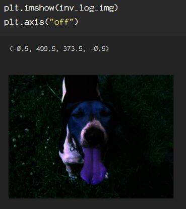
The inverse log transform is applied by creating the scaling constant, applying the transformation to the image, then converting the floats to integers(0,256).

This image is super dark, and is not the type of image that benefits from the inverse log transform in this state, but this can be useful in other circumstances.
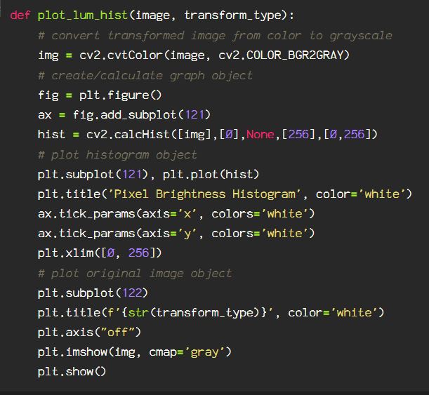
Using cv2.calcHist(), using the code block for plotting the histogram for the original image at the beginning of this post, creating a function to plot a histogram, I am able to plot for each of the power transformed images.
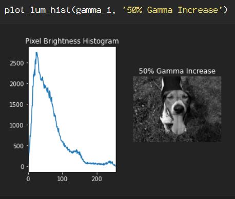
For the Gamma correction increase by 50%:
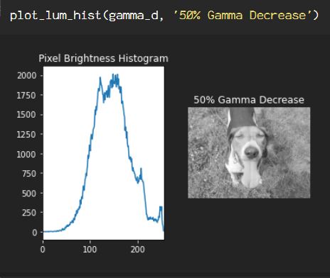
For the Gamma correction decrease by 50%:
For the log power transformation:

For the inverse power transformation:
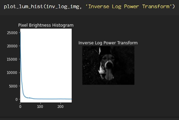
Image enhancement and restoration can be the end product, or it can be the beginning of the process, depending on the application. Don’t forget to check out the OpenCV documentation to get more info on the techniques shown here and more.
