Bag of Words to Term Frequency-Inverse Document Frequency and how it’s used in Natural Language Processing tasks.
When working on a dataset composed of words, first, the data is cleaned up, which makes up roughly 80 percent of the time spent on a given project. Every dataset is different as far as what steps are taken to clean it up, maybe you have removed stopwords, tokenized, lemmatized, stemmed, removed punctuation, whatever you do to get your data to a point where it’s a bit less bulky streamlined, in order to avoid wasting copious amounts of time processing unnecessarily, then we have to turn those words into something the computer can process.
Numbers are the language of computers, unlike the flourishes placed on words in French, or the excessive descriptions of descriptions in English, computers need these details turned into it’s native language. If the numbers are the language, then vectors are the sentences. Sometimes there is reason to assess character by character, but here, I am sticking to words.
Word2vec, Doc2Vec, GloVe are great options for generating representation vectors. Sometimes, however, all you need is the math for smaller datasets. When this happens, there are a couple of options.
For these examples, I am using a very small subset of a larger dataset. Obviously, this would be done on a large set of data in actual practice.
Option 1: The Bag-of-Words (BoW) method, where we take a document, and apply a term frequency count, where each time a term is used, we essentially apply ‘term’+=1 too the vector representing the document.
For this example, I am using Scikit Learn’s CountVectorizer(), the term frequency is calculated as follows:
tf-idf(t, d) = tf(t, d) * idf(t)


As you can see, there are 5 tweets, and cumulatively, there are 33 unique words present in the 5 tweets.
As you can see, the ‘features’ are each individual word. When assigning these 5 tweets I used as an example, to an array, this is what you see.

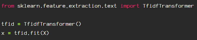
This is the TF in TF-IDF, which is why Scikit Learn has a TfidfTransformer() to pair up with the CountVectorizer(). Another option is to go straight for the TfidfVectorizer() should you be so inclined, as it combines these two steps into one step, simplifying the process, but for the sake of explanation, I will continue with the TfidfTransformer() to obtain the inverse document frequency:
idf(t) = log [ n / df(t) ] + 1
The + 1 at the end is added to avoid ignoring words with zero scores in the document, so it is slightly altered for scikit learn from the standard:
idf(t) = log [ n / (df(t) + 1) ]
I start by importing from Scikit Learn, then I assign and fit to my array of data that has been processed earlier with CountVectorizer(). The fit step is only done on the training data, the test data is transformed by the TfidfTransformer() that has been fit to the training data.
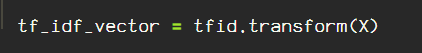
Next, transform the data.
To see the inverse document frequency weights for each word, put it into a dataframe for easy sorting capabilities, using the TfidfTransformer() assigned here as ‘tfid’, adding ‘.idf_’ to add the weights and then sort the values.
The inverse document frequency is taken from idf(w) = log (n
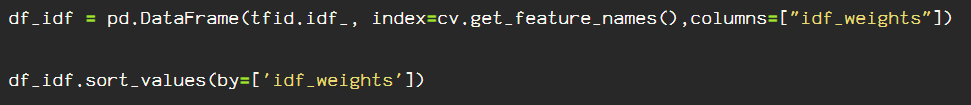
This is how it looks, all of the weights are present for the entire dataset.

Now, I am going back to my original feature names from my CountVectorizer(), to visualize the TF-IDF scores for the third tweet(I chose randomly) in my data by transposing to a dense matrix.

I create a DataFrame, and transpose, to a dense matrix, the third tweet, assigned to tweet_vector_2 above from the transformed training data. This can be done on unseen, testing data as well, skipping the ‘fit’ step.

And here, we have it, the TF-IDF scores for the third tweet in my data set.
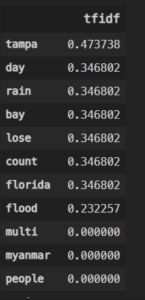
The tweet represented above, upon input to the transformer, looked like this:

There are a few ways to fine tune your TfidfTransformer() via optional parameters, such as ‘norm’, which can be set to’ l1′ or ‘l2’. There are a few other parameters that could be helpful in your data vectorization. Just check it out here.

Happy wording.
