
An audio file, or any sound really, has the following properties:
Frequency, Wavelength, Amplitude, Speed, Direction
These are characteristics that can be used to distinguish sounds from each other in neural networks, not unlike in the human brain.
Visualizing audio files is an important task in data science, due to the means of processing classification tasks. Extracted information and converting it to an image enables us to use computer vision type algorithms to compare and classify sounds.
First, we have to import librosa and matplotlib.
Initially, I created a dictionary by creating a dictionary from the lists I created, one with the file paths as strings, and the other with the name of the bird that is present in the audio clip by using the following line of code:
bird_dict = dict(zip(birds, audio_clips)) bird_dict = dict(zip(birds, audio_clips))
I am going to start with just plotting the waveform of the .wav files. In order to do this, the audio samples must be in .wav format, as .mp3 is not a recognized format in librosa. To plot this, the audio file is loaded and displayed via librosa

I am using the bird_dict dictionary that I created to iterate through the files and bird names for the titles on their respective waveforms.
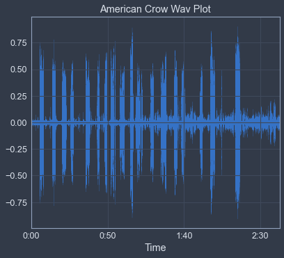
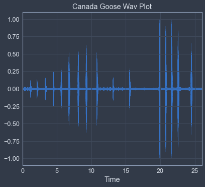
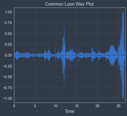
Now, as you can see, each of the waveforms look very different, as they are all different species of birds. The waveform plots the amplitude envelope over time, or the pressure of the sound as seen in the peaks from the origin up in crests and down in the troughs of the wave(form). It’s the power behind the sound, if you will. The wavelength is the distance from a specific point of height on the wav to the next spot on the wave where that exact value occurs on the same axis, at the same height, going in a constant direction from a temporal perspective. This doesn’t have to be any particular predetermined point, just a specific, constant point.

Next, the spectrogram is used to display frequency over time, measured in Hertz, or Hz. Frequency is exactly what it sounds like, how many cycles or vibrations repeat per second. The inverse of wavelength, longer wavelengths are the result of lower frequencies, and shorter wavelengths are the result of higher frequencies.
Before displaying the spectrogram, using librosa, the audio time series amplitude is converted to decibels after being transformed by obtaining the STFT (Short time Fourier transform) creating the variable “D” above. The y-axis argument should be ‘log’ to display the spectrogram as logarithmic.


This can also be shown linearly, however, due to the variation of frequencies that birds are capable of creating, the low frequencies are more obvious in a logarithmic scale. Humans perceive sound logarithmically, rather than in a linear fashion.
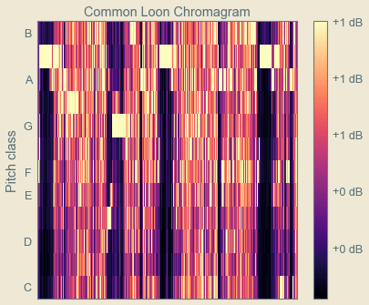
Next, the chromagram, which visually conveys the pitch profile of a sound, where it falls in the chromatic scale. The human brain processes sounds of the same chroma, occurring at different tone heights, or octaves, as related as a physiological response.


for k,v in bird_dict.items():
plot_chromagram(k,v) 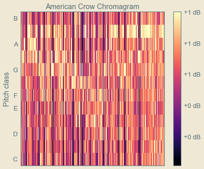

Librosa provides a plethora of other variations on these, as well as the ability to control the STFT variables like window_length, hop_length, and n_fft, and there are always wavelets to dive into later, but this provides the basic framework to create train/test data for audio classification in neural networks.
