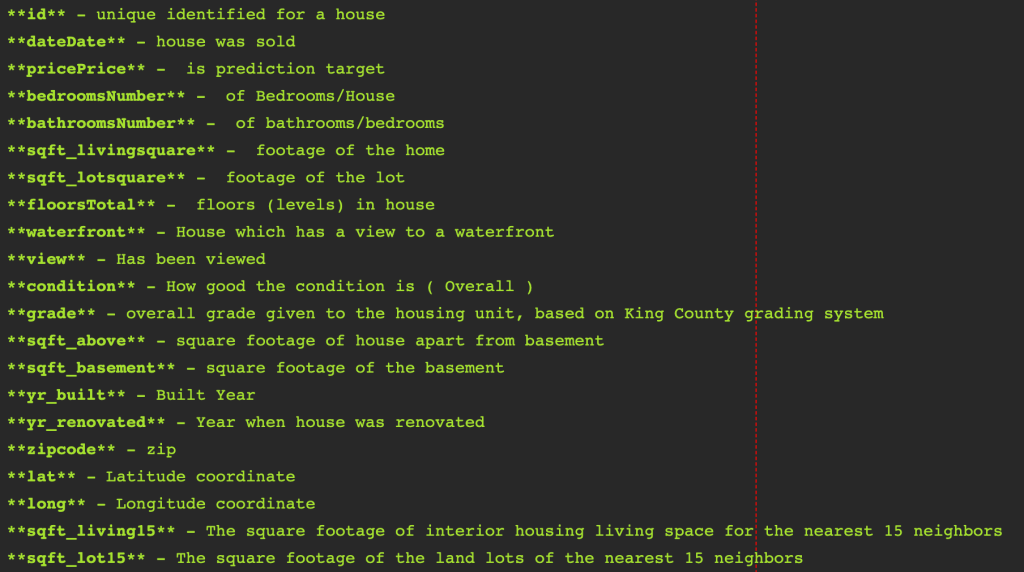
My motivation for the analysis of the King County Housing Dataset is a project for Module 2 of the Flatiron School Data Science program. I was provided a dataset with the below information included.
To start off, I began researching and assessing the dataset. I began by going to the King County, Washington website, https://info.kingcounty.gov/. Here, I found the Residential Glossary of Terms with information regarding the dataset.
Deciding, first, to drop the ‘views’ column, as I do not want my analysis to be tainted by the number of viewings of the properties, as that can be affected by many outside factors, such as realtor’s preferences, buyer curiosity, etc. The number of viewings does not suffice as any sort of accurate predictor or indicator.
Additionally, I reviewed the documentation on ‘grade’. Homes that have grades between 1 and 5 do not meet building code by law. Due to this information, I dropped homes falling below this specification, as I am only including homes that are fit to live in for this assessment. The lower graded homes are more consistent in their value and the higher grades, 11-13 have a wide range of price values but there are fewer occurrences of these grade values occurring overall.

Next, I assessed the ‘condition’ column, and due to the documentation on this description, I dropped any homes rating 1 or 2, only accepting average (needing work, still), and better homes.
I have also opted to drop the “waterfront” information, as there were several NaN values, which could indicate that it is not a waterfront property, but many of the properties already had a “0” for this, as this is already a binary column. To avoid misinterpreting the missing values, as there are 2,376, I simply dropped the column completely.
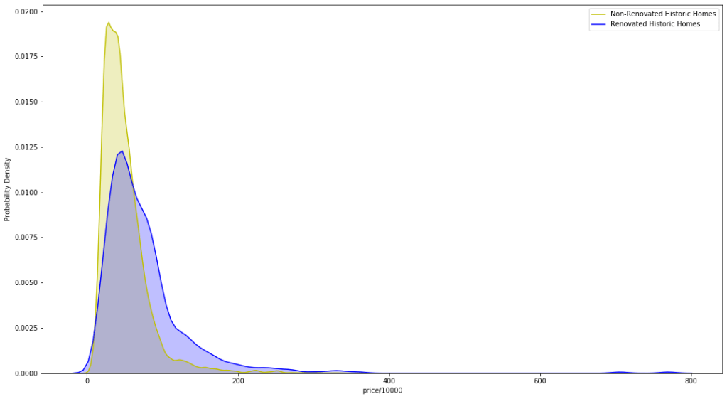
The “yr_renovated” column also had several missing values, which I interpret as these homes having not been renovated, so I replaced these with “0”. Using this information, I assessed what occurred to my target variable(‘price’) under circumstances where home was renovated vs not renovated. Finding that should the home be renovated, one can price the home over $60,000 higher than those homes of similar grades are priced.
I extracted the year of sale from the ‘date’ column, by converting to DateTime object, then using the year the property was sold and the ‘yr_built’ column, I calculated the age of each property. Then assessed the possible ‘historic’ homes, which, according to the state of Washington, is 50 years old and greater, and retaining the original structure and aesthetics. Since I could not assess the aesthetics, I simply assessed the renovated historic homes vs the non renovated historic homes as far as value. The renovated homes tend to fetch a higher price on a fairly consistent basis.
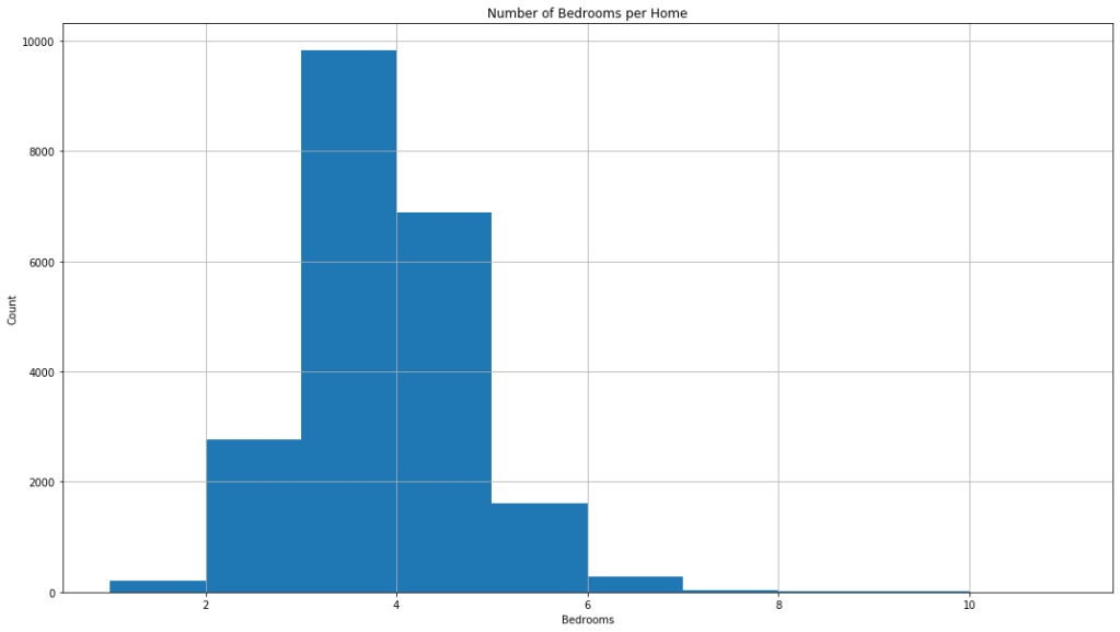
Next, I began my assessment of the features starting with the bedroom count. There seemed to be some typo errors present, which I corrected, and found that the most common home has 3 bedrooms, followed by 4 bedrooms.
The dataset provided was not in metric values, rather it was in the english system, so I converted all measurements from square feet to square meters.

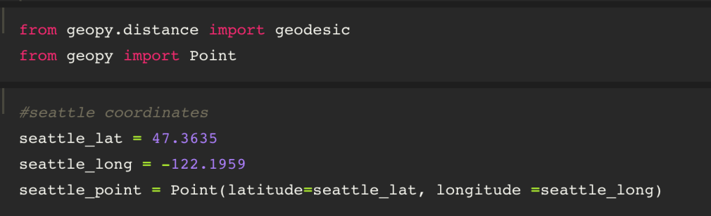
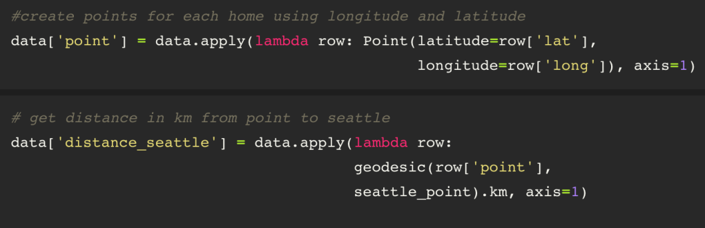
Deciding to utilize the longitude and latitude information provided, I obtained the latitude and longitude coordinates for the nearest city, Seattle, the used geopy to convert the latitudes and longitudes to a point so that I could calculate the distance from each home listed to the city of Seattle(using kilometers, of course).
I, then assessed the zipcode column and created a graph to visualize the zipcodes and the mean price of homes in each zipcode, before removing the column, along with the ‘lat’ and ‘long’ columns.

Once I finished cleaning up my dataset, removing the english system measurement data, I began my assessment of my target variable, ‘price’.
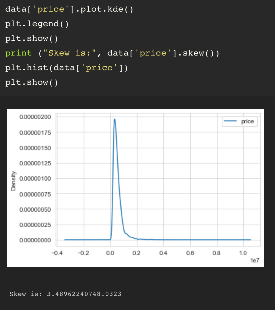
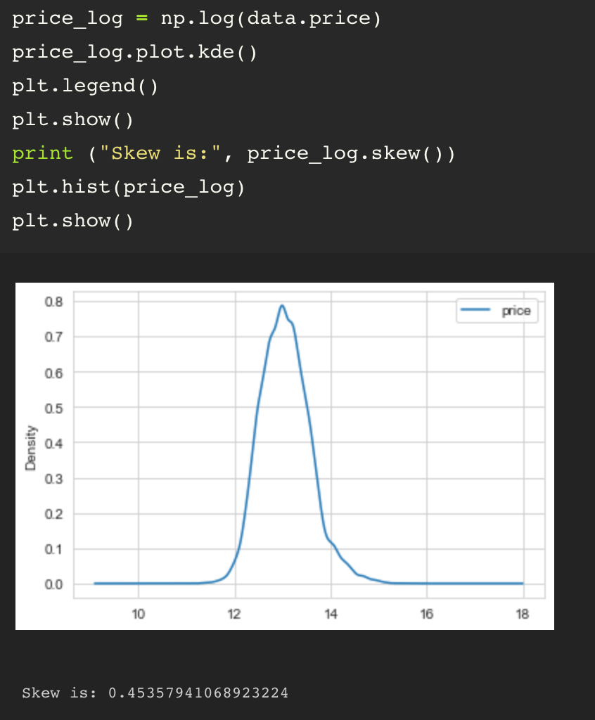
Due to the fact that the price data is not a normal distribution, I tried a couple different options to scale and normalize the distribution and ended up setting on taking the log of the price values for my assessment.
Some columns that I dropped throughout my assessment include ‘floors’, ‘sqm_lot15’, ‘views’, ‘waterfront’, ‘lat’, ‘long’, ‘date’, ‘yr_renovated’, ‘yr_built’, and ‘zipcode’. Some of these were used to create new data(really, data from a different perspective), some were irrelevant, and others were simply redundant.
Once I completed my data scrubbing and cleaning. I used my variables to get an idea of where I stood on my regression before processing the categorical variables such as bedrooms, bathrooms, condition and grade.
As predicted, there are some issues with some of the data, so I created dummy variables for the categorical data. Rather than keeping all of the quarter and half bathroom values as decimals, I rounded the bathroom values before creating dummy variables(I actually did this both ways and rounding had no negative effect, but allowed me to work with fewer dummy variables). For the dummy variables, I dropped the first variable for each category to ensure I avoided the dummy variable trap.

My continuous data, are as follows: square meters living area(‘sqm_living’), square meters living area of the 15 nearest neighbors(‘sqm_living15’), square meter lot size(‘sqm_lot’), distance to seattle(‘distance_seattle’), and age variables.
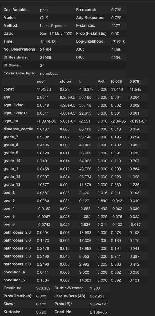
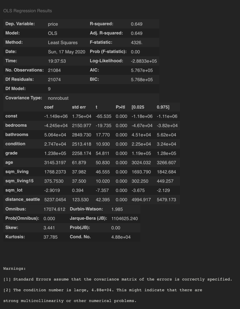
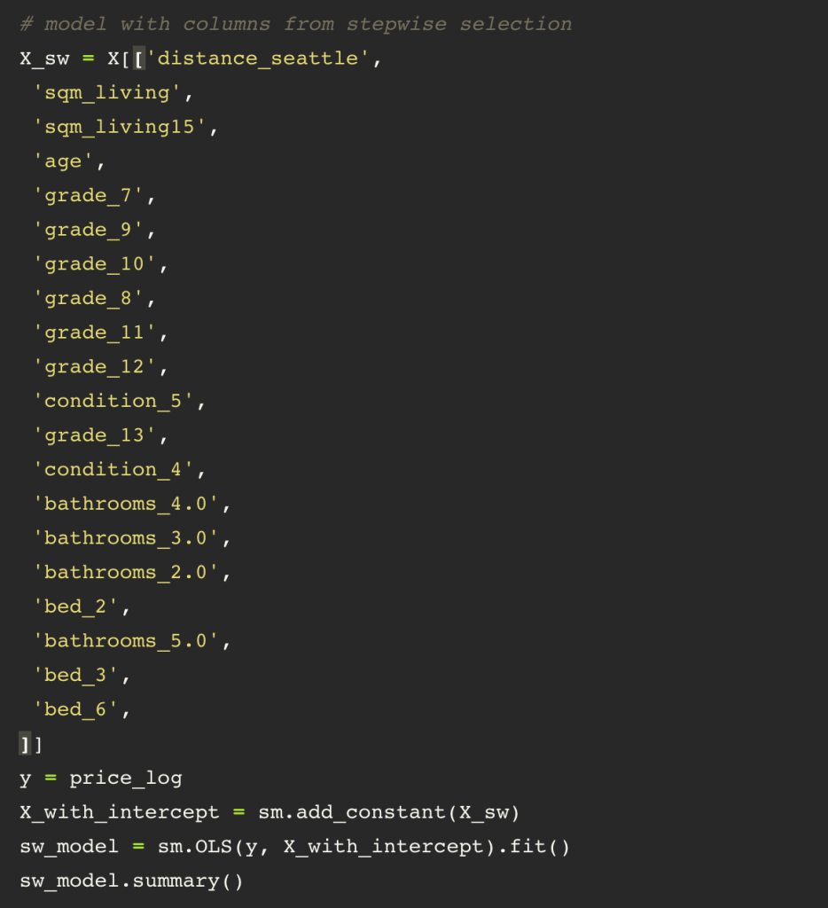
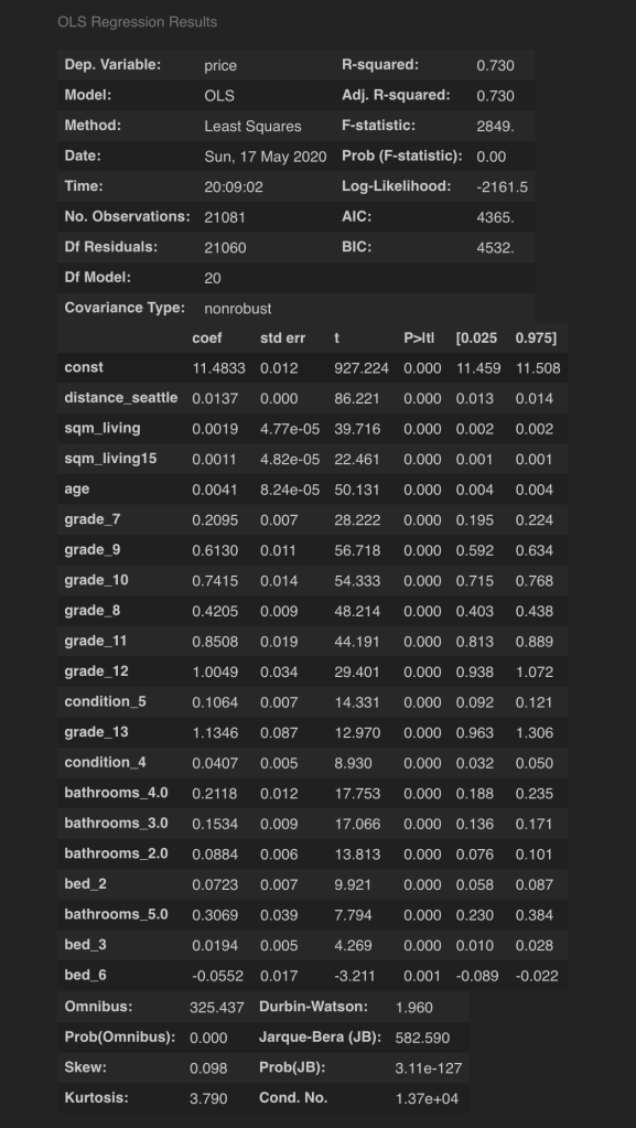
Getting closer to where I need to be with this model. I am going to drop the sqm_lot column from my next model. Now I perform stepwise selection based on my p-values to decide what columns to keep.
I then split my data and create a model in scikit learn using the same data.

My model is still overshooting predictions.

To further hone in on the accuracy of the model in the future, I will probably run the square meter data through the StandardScaler() and assess the other continuous data to decide what my best option is for it as well. Additional work as far as Polynomial Regression for the independent variables should also be explored.
